pROC has always accepted ordered factors as predictors (for example aSAH$wfns, the WFNS neurological grade in the aSAH dataset, with levels 1 to 5). Internally it simply called as.numeric() on them and computed thresholds as the midpoints between consecutive numeric codes (1.5, 2.5, and so on).

That's reasonable when the levels happen to be the numbers 1:n, but it is not appropriate for an ordered factor whose levels are textual, for example "very low", "low", "medium", "high", "very high". The thresholds were still -Inf, 1.5, 2.5, 3.5, 4.5, Inf, numbers that do not correspond to anything in the data and are meaningless to show. This was reported as issue #63, and a fix for it was just merged into the develop branch.

In practice, this could potentially break some of your code. Before it reaches CRAN, I'd like testers who use ordered predictors to try the develop version on their own data and tell me if anything looks wrong.

What changes

On develop, thresholds of an ordered ROC curve are now the predictor's own levels, plus one infinite sentinel for the all-positive or all-negative cut-off. Sensitivities, specificities and AUC are exactly the same as before, only the threshold labels change, from numeric midpoints to the levels you actually gave it:

library(pROC)
data(aSAH)

wfns.txt <- aSAH$wfns
levels(wfns.txt) <- c("very low", "low", "medium", "high", "very high")

r <- roc(aSAH$outcome, wfns.txt, quiet = TRUE)
r$thresholds
# very low, low, medium, high, very high, Inf
# Levels: very low < low < medium < high < very high < Inf

coords(r, "medium")
#   threshold specificity sensitivity
# 1    medium   0.7916667   0.6585365

This is a breaking change for any code that reads roc$thresholds as numbers, or passes a numeric cut-off into coords(), ci.thresholds(), ci.coords(), or plot.roc(print.thres = ...) on an ordered ROC curve. Numeric predictors are entirely unaffected by this change. Where you used to pass a midpoint, pass the level label instead:

# Incorrect (pROC <= 1.19.1 converted wfns to 1:5, thresholds were midpoints):
coords(roc(aSAH$outcome, aSAH$wfns), 2.5)

# Correct: pass the level label
coords(roc(aSAH$outcome, aSAH$wfns, quiet = TRUE), "3")

The mapping from old midpoints to new labels is straightforward (for direction = "<", the default): the old -Inf becomes the lowest level, the old midpoint k + 0.5 becomes the level in position k + 1, and the old Inf becomes the level literally named "Inf".

As a side effect of the same fix, ci.coords(..., x = "best", best.policy = "omit") now correctly drops a bootstrap replicate that has several equally-good "best" points, instead of silently keeping the first one.

How to test it

This is not released yet: it is only on the develop branch, ahead of the next CRAN release, planned for early 2027. If you use ordered predictors with roc(), please install the development version and run your own code against it:

if (! requireNamespace("devtools")) install.packages("devtools")
devtools::install_github("xrobin/pROC@develop")

Recommendations

If you have scripts or packages that build ROC curves from ordered predictors, please run them against the develop version and check the following:

• Any place you hard-code a numeric threshold for an ordered predictor (in coords(), ci.thresholds(), ci.coords(), or print.thres) will need to switch to the level label.
• roc() now requires cases and controls built from ordered vectors to have identical levels; it errors instead of silently coercing when they differ (for example after an unbalanced droplevels()).
• Smoothing an ordered ROC curve now only supports method = "binormal"; other smoothing methods error instead of silently falling back to a numeric conversion.
• AUC, DeLong and bootstrap CIs, roc.test(), cov()/var(), and power.roc.test() all still match what you got before. Only the thresholds changed, not the statistics.

If anything looks off, please comment on issue #63 or open a new issue on GitHub before this reaches CRAN. Thanks in advance for testing!

pROC 1.19.1 is a minor maintenance release. The only user-facing change is the introduction of a FAQ vignette which supersedes the old wiki.

Here is the full changelog:

• Added a FAQ vignette
• Removed unused tcltk from Suggests
• Tests now skip if Suggest'ed packages are missing
• Fix CRAN checks NOTE about structure() special names (.Names, .Dim, .Dimnames)

pROC version 1.19.0 was just released and will be available on CRAN very soon.

Besides minor changes and fixes in the coords and ci.coords functions, the main updates in this version focus on the core of the package, aiming to make it more modern, efficient, and easier to maintain. Several features that were difficult to maintain have been deprecated.

• The dependency on the retired plyr package has been removed (thanks to Michael Chirico for his contributions). Unfortunately, as a side effect, progress bars and parallel processing have been removed. Trying to set the progress and parallel arguments will now trigger a warning, and the arguments will be ignored.
• As a followup from the changes to the output of the coords function in version 1.16.0, the transpose, as.list, as.matrix and drop arguments have been deprecated. The coords function currently has multiple exit points, depending on arguments and inputs, and can return retults in mutliple formats. This makes it difficult to use and to maintain. Going forward, coords will only retrun data in a single, tidy data.frame format, compatible following modern R coding practices. For compatibility reasons, deprecated arguments are still available, but setting them to non default values will trigger warnings. They will be removed in a future release. If your code still uses these arguments, please update it accordingly.
• Finally, following years of performance improvements, an in an effort to simplify the codebase, all ROC computation algorithms other than 2 have been removed as they no longer provided meaningful performance advantages. The algorithm argument to roc has been deprecated. Setting it to a non-default value has no effect and triggers a warning. The fun.sesp value of roc objects is also deprecated. Calling it triggers a warning. Both will be removed in a future release of pROC.

Here is the full changelog:

• ci.coords can now take the same input values as coords (issue #90)
• ci.coords can be plotted
• Added "lr_pos" and "lr_neg" to coords (issue #102)
• coords with partial.auc now interpolates bounds when needed
• Added ignore.partial.auc argument to coords
• Deprecated transpose, as.list, as.matrix and drop in coords
• Deprecated the algorithm argument to roc and fun.sesp value
• Deprecated the progress and parallel argument for bootstrap operations.
• Removed dependencies on doParallel and retired package plyr (thanks to Michael Chirico, pr #134, #135, #136, #137, #138, #139 and #140).

You can update your installation by simply typing:

install.packages("pROC")

Update: pROC 1.19.0 was rejected from CRAN. A patch revision 1.19.0.1 was created to workaround an issue with a reverse dependency but provides no meaningful change:

• Move fun.sesp definition to work around LudvigOlsen/cvms#44.

pROC 1.18.5 is now available on CRAN. It's a minor bugfix release:

• Fixed formula input when given as variable and combined with with (issue #111)
• Fixed formula containing variables with spaces (issue #120)
• Fixed broken grouping when colour argument was given in ggroc (issue #121)

You can update your installation by simply typing:

install.packages("pROC")

In this document I am going create a video showing the training of the inner-most layer of Deep Belief Network (DBN) using the MNIST dataset of handwritten digits. I will use our DeepLearning R package that implements flexible DBN architectures with an object-oriented interface.

MNIST

The MNIST dataset is a database of handwritten digits with 60,000 training images and 10,000 testing images. You can learn everything about it on Wikipedia. In short, it is the go-to dataset to train and test handwritten digit recognition machine learning algorithms.

I made an R package for easy access, named mnist. The easiest way to install it is with devtools. If you don't have it already, let's first install devtools:

if (!require("devtools")) {install.packages("devtools")}

Now we can install mnist:

devtools::install_github("xrobin/mnist")

PCA

In order to see what the dataset looks like, let's use PCA to reduce it to two dimensions.

pca <- prcomp(mnist$train$x)
plot.mnist(
	prediction = predict(pca, mnist$test$x),
	reconstruction = tcrossprod(
		predict(pca, mnist$test$x)[,1:2], pca$rotation[,1:2]),
	highlight.digits = c(72, 3, 83, 91, 6688, 7860, 92, 1, 180, 13))

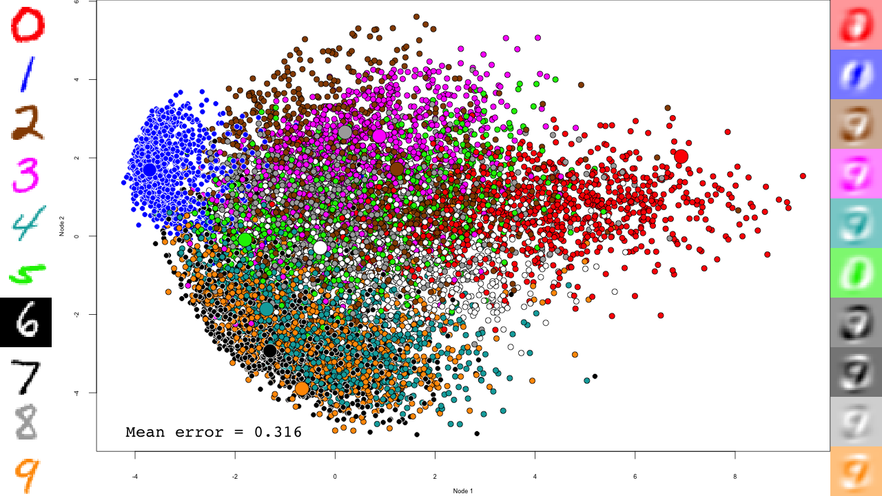
Let's take a minute to describe this plot. The central scatterplot shows first two components of the PCA of all digits in the test set. On the left hand side, I picked 10 representative digits from the test set to highlight, which are shown as larger circles in the central scatterplot. On the left are the "reconstructed digits", which were reconstructed from the two first dimensions of the PCA. While we can see some digit-like structures, it is basically impossible to recognize them. We can see some separation of the digits in the 2D space as well, but it is pretty weak and some pairs cannot be distinguished at all (like 4 and 9). Of course the reconstructions would look much better had we kept all PCA dimensions, but so much for dimensionality reduction.

Deep Learning

Now let's see if we can do better with Deep Learning. We'll use a classical Deep Belief Network (DBN), based on Restricted Boltzmann Machines (RBM) similar to what Hinton described back in 2006 (Hinton & Salakhutdinov, 2006). The training happens in two steps: a pre-training step with contrastive divergence stochastic gradient descent brings the network to a reasonable starting point for a more conventional conjugate gradient optimization (hereafter referred to as fine-tuning).

I implemented this algorithm with a few modifications in an R package which is available on GitHub. The core of the processing is done in C++ with RcppEigen (Bates & Eddelbuettel, 2013) for higher speed. Using devtools again:

devtools::install_github("xrobin/DeepLearning")

We will use this code to train a 5 layers deep network, that reduces the digits to an abstract, 2D representation. By looking at this last layer throughout the training process we can start to understand how the network learns to recognize digits. Let's start by loading the required packages and the MNIST dataset, and create the DBN.

library(DeepLearning)
library(mnist)
data(mnist)

dbn <- DeepBeliefNet(Layers(c(784, 1000, 500, 250, 2),
	input = "continuous", output = "gaussian"),
	initialize = "0")

We just created the 5-layers DBN, with continuous, 784 nodes input (the digit image pixels), and a 2 nodes, gaussian output. It is initialized with 0, but we could have left out the initialize to start from a random initilization (Bengio et al., 2007). Before we go, let's define a few useful variables:

output.folder <- "video" # Where to save the output
maxiters.pretrain <- 1e6  # Number of pre-training iterations
maxiters.train <- 10000 # Number of fine-tuning iterations
run.training <- run.images <- TRUE # Turn any of these off 
# Which digits to highlight and reconstruct
highlight.digits = c(72, 3, 83, 91, 6688, 7860, 92, 1, 180, 13)

We'll also need the following function to show the elapsed time:

format.timediff <- function(start.time) {
    diff = as.numeric(difftime(Sys.time(), start.time, units="mins"))
    hr <- diff%/%60
    min <- floor(diff - hr * 60)
    sec <- round(diff%%1 * 60,digits=2)
    return(paste(hr,min,sec,sep=':'))
}

Pre-training

Initially, the network is a stack of RBMs that we need to pre-train one by one. Hinton & Salakhutdinov (2006) showed that this step is critical to train deep networks. We will use 1000000 iterations (maxiters.pretrain) of contrastive divergence, which takes a couple of days on a modern CPU. Let's start with the first three RBMs:

First three RBMs

if (run.training) {
	sprintf.fmt.iter <- sprintf("%%0%dd", nchar(sprintf("%d", maxiters.pretrain)))
	
	mnist.data.layer <- mnist
	for (i in 1:3) {

We define a diag function that will simply print where we are in the training. Because this function will be called a million times (maxiters.pretrain), we can use rate = "accelerate" to slow down the printing over time and save a few CPU cycles.

		diag <- list(rate = "accelerate", data = NULL, f = function(rbm, batch, data, iter, batchsize, maxiters, layer) {
			print(sprintf("%s[%s/%s] in %s", layer, iter, maxiters, format.timediff(start.time)))
		})

We can get the current RBM, and we will work on it directly. Let's save it for good measure, as well as the current time for the progress function:

		rbm <- dbn[[i]]
		save(rbm, file = file.path(output.folder, sprintf("rbm-%s-%s.RData", i, "initial")))
		start.time <- Sys.time()

Now we can start the actual pre-training:

		rbm <- pretrain(rbm, mnist.data.layer$train$x,
			penalization = "l2", lambda=0.0002, momentum = c(0.5, 0.9),
			epsilon=c(.1, .1, .1, .001)[i], batchsize = 100, maxiters=maxiters.pretrain,
			continue.function = continue.function.always, diag = diag)

This can take some time, especially for the first layers which are larger. Once it is done, we predict the data through this RBM for the next layer and save the results:

		mnist.data.layer$train$x <- predict(rbm, mnist.data.layer$train$x)
		mnist.data.layer$test$x <- predict(rbm, mnist.data.layer$test$x)
		save(rbm, file = file.path(output.folder, sprintf("rbm-%s-%s.RData", i, "final")))
		dbn[[i]] <- rbm
	}

Last RBM

This is very similar to the previous three, but note that we save the RBM within the diag function. We could generate the plot directly, but it is easier to do it later once we have some idea about the final axis we will need. Please note the rate = "accelerate" here. You probably don't want to save a million RBM objects on your hard drive, both for speed and space reasons.

	rbm <- dbn[[4]]
	print(head(rbm$b))
	diag <- list(rate = "accelerate", data = NULL, f = function(rbm, batch, data, iter, batchsize, maxiters, layer) {
		save(rbm, file = file.path(output.folder, sprintf("rbm-4-%s.RData", sprintf(sprintf.fmt.iter, iter))))
		print(sprintf("%s[%s/%s] in %s", layer, iter, maxiters, format.timediff(start.time)))
	})
	save(rbm, file = file.path(output.folder, sprintf("rbm-%s-%s.RData", 4, "initial")))
	start.time <- Sys.time()
	rbm <- pretrain(rbm, mnist.data.layer$train$x,  penalization = "l2", lambda=0.0002,
		epsilon=.001, batchsize = 100, maxiters=maxiters.pretrain,
		continue.function = continue.function.always, diag = diag)
	save(rbm, file = file.path(output.folder, sprintf("rbm-4-%s.RData", "final")))
	dbn[[4]] <- rbm

If we were not querying the last layer, we could have pre-trained the entire network at once with the following call:

	dbn <- pretrain(dbn, mnist.data.layer$train$x, 
		penalization = "l2", lambda=0.0002, momentum = c(0.5, 0.9),
		epsilon=c(.1, .1, .1, .001), batchsize = 100, 
		maxiters=maxiters.pretrain,
		continue.function = continue.function.always)

Pre-training parameters

Pre-training RBMs is quite sensitive to the use of proper parameters. With improper parameters, the network can quickly go crazy and start to generate infinite values. If that happens to you, you should try to tune one of the following parameters:

• penalization: this is the penalty of introducing or increasing the value of a weight. We used L2 regularization, but "l1" is available if a sparser weight matrix is needed.
• lambda: the regularization rate. In our experience 0.0002 works fine with the MNIST and other datasets of similar sizes such as cellular imaging data. Too small or large values will result in over- or under-fitted networks, respectively.
• momentum: helps avoiding oscillatory behaviors, where the network oscillate between iterations. Allowed values can range from 0 (no momentum) to 1 (full momentum = no training). Here we used an increasing gradient of momentum which starts at 0.5 and increases linearly to 0.9, in order to stabilize the final network without compromising early training steps.
• epsilon: the learning rate. Typically, 0.1 works well with binary and continuous output layers, and must be decreased to around 0.001 for gaussian outputs. Too large values will drive the network to generate infinities, while too small ones will slow down the training.
• batchsize: larger batch sizes will result in smoother but slower training. Small batch sizes will make the training "jumpy", which can be compensated by lower learning rates (epsilon) or increased momentum.

Fine-tuning

This is where the real training happens. We use conjugate gradients to find the optimal solution. Again, the diag function saves the DBN. This time we use rate = "each" to save every step of the training. First we have way fewer steps, but also the training itself happen at a much more stable speed than in the pre-training, where things slow down dramatically.

	sprintf.fmt.iter <- sprintf("%%0%dd", nchar(sprintf("%d", maxiters.train)))
	diag <- list(rate = "each", data = NULL, f = function(dbn, batch, data, iter, batchsize, maxiters) {
		save(dbn, file = file.path(output.folder, sprintf("dbn-finetune-%s.RData", sprintf(sprintf.fmt.iter, iter))))
		print(sprintf("[%s/%s] in %s", iter, maxiters, format.timediff(start.time)))
	})
	save(dbn, file = file.path(output.folder, sprintf("dbn-finetune-%s.RData", "initial")))
	start.time <- Sys.time()
	dbn <- train(unroll(dbn), mnist$train$x, batchsize = 100, maxiters=maxiters.train,
		continue.function = continue.function.always, diag = diag)
	save(dbn, file = file.path(output.folder, sprintf("dbn-finetune-%s.RData", "final")))
}

And that's it, our DBN is now fully trained!

Generating the images

Now we need to read in the saved network states again, pass the data through the network (predict) and save this in HD-sized PNG file.

The first three RBMs are only loaded into the DBN

if (run.images) {
	for (i in 1:3) {
		load(file.path(output.folder, sprintf("rbm-%d-final.RData", i)))
		dbn[[i]] <- rbm
	}

The last RBM is where interesting things happen.

	for (file in list.files(output.folder, pattern = "rbm-4-.+\\.RData", full.names = TRUE)) {
		print(file)
		load(file)
		dbn[[4]] <- rbm
		iter <- stringr::str_match(file, "rbm-4-(.+)\\.RData")[,2]

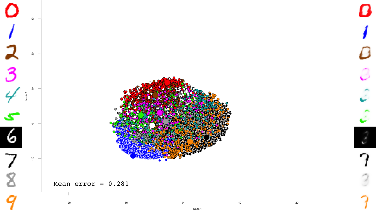
We now predict and reconstruct the data, and calculate the mean reconstruction error:

		predictions <- predict(dbn, mnist$test$x)
		reconstructions <- reconstruct(dbn, mnist$test$x)
		iteration.error <- errorSum(dbn, mnist$test$x) / nrow(mnist$test$x)

Now the actual plotting. Here I selected xlim and ylim values that worked well for my training run, but your mileage may vary.

		png(sub(".RData", ".png", file), width = 1280, height = 720) # hd output
		plot.mnist(model = dbn, x = mnist$test$x, label = mnist$test$y+1, predictions = predictions, reconstructions = reconstructions,
				   ncol = 16, highlight.digits = highlight.digits,
				   xlim = c(-12.625948, 8.329168), ylim = c(-10.50657, 13.12654))
		par(family="mono")
		legend("bottomleft", legend = sprintf("Mean error = %.3f", iteration.error), bty="n", cex=3)
		legend("bottomright", legend = sprintf("Iteration = %s", iter), bty="n", cex=3)
		dev.off()
	}

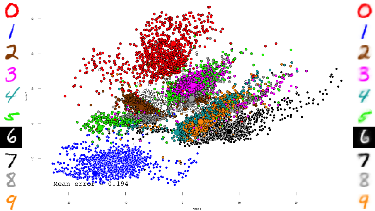
We do the same with the fine-tuning:

	for (file in list.files(output.folder, pattern = "dbn-finetune-.+\\.RData", full.names = TRUE)) {
		print(file)
		load(file)
		iter <- stringr::str_match(file, "dbn-finetune-(.+)\\.RData")[,2]
		predictions <- predict(dbn, mnist$test$x)
		reconstructions <- reconstruct(dbn, mnist$test$x)
		iteration.error <- errorSum(dbn, mnist$test$x) / nrow(mnist$test$x)
		png(sub(".RData", ".png", file), width = 1280, height = 720) # hd output
		plot.mnist(model = dbn, x = mnist$test$x, label = mnist$test$y+1, predictions = predictions, reconstructions = reconstructions,
				   ncol = 16, highlight.digits = highlight.digits,
				   xlim = c(-22.81098,  27.94829), ylim = c(-17.49874,  33.34688))
		par(family="mono")
		legend("bottomleft", legend = sprintf("Mean error = %.3f", iteration.error), bty="n", cex=3)
		legend("bottomright", legend = sprintf("Iteration = %s", iter), bty="n", cex=3)
		dev.off()
	}
}

The video

I simply used ffmpeg to convert the PNG files to a video:

cd video
ffmpeg -pattern_type glob -i "rbm-4-*.png" -b:v 10000000 -y ../rbm-4.mp4
ffmpeg -pattern_type glob -i "dbn-finetune-*.png" -b:v 10000000 -y ../dbn-finetune.mp4

And that's it! Notice how the pre-training only brings the network to a state similar to that of a PCA, and the fine-tuning actually does the separation, and how it really makes the reconstructions accurate.

Application

We used this code to analyze changes in cell morphology upon drug resistance in cancer. With a 27-dimension space, we could describe all of the observed cell morphologies and predict whether a cell was resistant to ErbB-family drugs with an accuracy of 74%. The paper is available in Open Access in Cell Reports, DOI 10.1016/j.celrep.2020.108657.

Concluding remarks

In this document I described how to build and train a DBN with the DeepLearning package. I also showed how to query the internal layer, and use the generative properties to follow the training of the network on handwritten digits.

DBNs have the advantage over Convolutional Networks (CN) that they are fully generative, at least during the pre-training. They are therefore easier to query and interpret as we have demonstrated here. However keep in mind that CNs have demonstrated higher accuracies on computer vision tasks, such as the MNIST dataset.

Additional algorithmic details are available in the doc folder of the DeepLearning package.

References

Our paper, 2021

Longden J., Robin X., Engel M., et al. Deep neural networks identify signaling mechanisms of ErbB-family drug resistance from a continuous cell morphology space. Cell Reports, 2021;34(3):108657.

Bates & Eddelbuettel, 2013

Bates D, Eddelbuettel D. Fast and Elegant Numerical Linear Algebra Using the RcppEigen Package. Journal of Statistical Software, 2013;52(5):1–24.

Bengio et al., 2007

Bengio Y, Lamblin P, Popovici D, Larochelle H. Greedy layer-wise training of deep networks. Advances in neural information processing systems. 2007;19:153–60.

Hinton & Salakhutdinov, 2006

Hinton GE, Salakhutdinov RR. Reducing the Dimensionality of Data with Neural Networks. Science. 2006;313(5786):504–7.

Downloads

1. Code to generate the video
2. DeepLearning package source code

pROC version 1.18.0 is now available on CRAN now. Only a few changes were implemented in this release:

• Add CI of the estimate for roc.test (DeLong, paired only for now) (code contributed by Zane Billings) (issue #95).
• Fix documentation and alternative hypothesis for Venkatraman test (issue #92).

You can update your installation by simply typing:

install.packages("pROC")

pROC version 1.17.0.1 is available on CRAN now. Besides several bug fixes and small changes, it introduces more values in input of coords.

Here is an example:

library(pROC)
data(aSAH)
rocobj <- roc(aSAH$outcome, aSAH$s100b)
coords(rocobj, x = seq(0, 1, .1), input="recall", ret="precision")
#    precision
# 1        NaN
# 2  1.0000000
# 3  1.0000000
# 4  0.8601399
# 5  0.6721311
# 6  0.6307692
# 7  0.6373057
# 8  0.4803347
# 9  0.4517906
# 10 0.3997833
# 11 0.3628319

Getting the update

The update his available on CRAN now. You can update your installation by simply typing:

install.packages("pROC")

Here is the full changelog:

1.17.0.1 (2020-01-07):

• Fix CRAN incoming checks as requested by CRAN.

1.17.0 (2020-12-29)

• Accept more values in input of coords (issue #67).
• Accept kappa for the power.roc.test of two ROC curves (issue #82).
• The input argument to coords for smooth.roc curves no longer has a default.
• The x argument to coords for smooth.roc can now be set to all (also the default).
• Fix bootstrap roc.test and cov with smooth.roc curves.
• The ggroc function can now plot smooth.roc curves (issue #86).
• Remove warnings with warnPartialMatchDollar option (issue #87).
• Make tests depending on vdiffr conditional (issue #88).

pROC version 1.16.1 is a minor release that disables a timing-dependent test based on the microbenchmark package that can sometimes cause random failures on CRAN. This version contains no user-visible changes. Users don't need to install this update.

pROC version 1.16.0 is available on CRAN now. Besides several bug fixes, the main change is the switch of the default value of the transpose argument to the coords function from TRUE to FALSE. As announced earlier, this is a backward incompatible change that will break any script that did not previously set the transpose argument and for now comes with a warning to make debugging easier. Scripts that set transpose explicitly are not unaffected.

New return values of coords and ci.coords

With transpose = FALSE, the coords returns a tidy data.frame suitable for use in pipelines:

data(aSAH)
rocobj <- roc(aSAH$outcome, aSAH$s100b)
coords(rocobj, c(0.05, 0.2, 0.5), transpose = FALSE)
#      threshold specificity sensitivity
# 0.05      0.05  0.06944444   0.9756098
# 0.2       0.20  0.80555556   0.6341463
# 0.5       0.50  0.97222222   0.2926829

The function doesn't drop dimensions, so the result is always a data.frame, even if it has only one row and/or one column.

If speed is of utmost importance, you can get the results as a non-transposed matrix instead:

coords(rocobj, c(0.05, 0.2, 0.5), transpose = FALSE, as.matrix = TRUE)
#      threshold specificity sensitivity
# [1,]      0.05  0.06944444   0.9756098
# [2,]      0.20  0.80555556   0.6341463
# [3,]      0.50  0.97222222   0.2926829

In some scenarios this can be a tiny bit faster, and is used internally in ci.coords.

Type help(coords_transpose) for additional information.

ci.coords

The ci.coords function now returns a list-like object:

ciobj <- ci.coords(rocobj, c(0.05, 0.2, 0.5))
ciobj$accuracy
#        2.5%       50%     97.5%
# 1 0.3628319 0.3982301 0.4424779
# 2 0.6637168 0.7433628 0.8141593
# 3 0.6725664 0.7256637 0.7787611

The print function prints a table with all the results, however this table is generated on the fly and not available directly.

ciobj
# 95% CI (2000 stratified bootstrap replicates):
#      threshold sensitivity.low sensitivity.median sensitivity.high
# 0.05      0.05          0.9268             0.9756           1.0000
# 0.2       0.20          0.4878             0.6341           0.7805
# 0.5       0.50          0.1707             0.2927           0.4390
#      specificity.low specificity.median specificity.high accuracy.low
# 0.05         0.01389            0.06944           0.1250       0.3628
# 0.2          0.70830            0.80560           0.8889       0.6637
# 0.5          0.93060            0.97220           1.0000       0.6726
#      accuracy.median accuracy.high
# 0.05          0.3982        0.4425
# 0.2           0.7434        0.8142
# 0.5           0.7257        0.7788

The following code snippet can be used to obtain all the information calculated by the function:

for (ret in attr(ciobj, "ret")) {
	print(ciobj[[ret]])
}
#        2.5%       50%     97.5%
# 1 0.9268293 0.9756098 1.0000000
# 2 0.4878049 0.6341463 0.7804878
# 3 0.1707317 0.2926829 0.4390244
#         2.5%        50%     97.5%
# 1 0.01388889 0.06944444 0.1250000
# 2 0.70833333 0.80555556 0.8888889
# 3 0.93055556 0.97222222 1.0000000
#        2.5%       50%     97.5%
# 1 0.3628319 0.3982301 0.4424779
# 2 0.6637168 0.7433628 0.8141593
# 3 0.6725664 0.7256637 0.7787611

Getting the update

The update his available on CRAN now. You can update your installation by simply typing:

install.packages("pROC")

Here is the full changelog:

• BACKWARD INCOMPATIBLE CHANGE: transpose argument to coords switched to FALSE by default (issue #54).
• BACKWARD INCOMPATIBLE CHANGE: ci.coords return value is now of list type and easier to use.
• Fix one-sided DeLong test for curves with direction=">" (issue #64).
• Fix an error in ci.coords due to expected NA values in some coords (like "precision") (issue #65).
• Ordrered predictors are converted to numeric in a more robust way (issue #63).
• Cleaned up power.roc.test code (issue #50).
• Fix pairing with roc.formula and warn if na.action is not set to "na.pass" or "na.fail" (issue #68).
• Fix ci.coords not working with smooth.roc curves.

A new version of pROC, 1.15.3, has been released and is now available on CRAN. It is a minor bugfix release. Versions 1.15.1 and 1.15.2 were rejected from CRAN.

Here is the full changelog:

• Fix -Inf threshold in coords for curves with direction = ">" (issue 60).
• Keep list order in ggroc (issue 58).
• Fix erroneous error in ci.coords with ret="threshold" (issue 57).
• Restore lazy loading of the data and fix an R CMD check warning "Variables with usage in documentation object 'aSAH' not in code".
• Fix vdiffr unit tests with ggplot2 3.2.0 (issue 53).